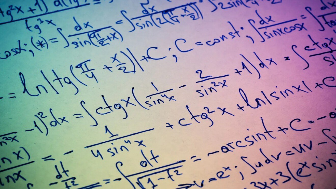
Differential equations are one of the most important branches of higher mathematics, studied by students at technical universities. At MEPhI this subject is traditionally taught in the second year and forms the basis for understanding many physical processes.
What a Differential Equation Is
A differential equation is an equation that, besides a function, also contains its derivatives. Unlike algebraic equations, where one seeks a number or several numbers, solving a differential equation means finding a function or family of functions.
The key difference between a differential equation and a simple mathematical expression is that not every equation containing derivatives of an unknown function is a differential equation. For example, the equation f′(x) = f(f(x)) is not a differential equation.
Classification of Differential Equations
By Order
The order of a differential equation is the highest order of derivative it contains. First- and second-order differential equations are of the greatest practical importance.
Example of a second-order, fourth-degree equation: (y″)⁴ + y′ + y⁶ + x⁷ = 0
By Type of Variable
- Ordinary differential equations (ODEs) — contain functions of only one argument
- Partial differential equations (PDEs) — the functions depend on several variables
- Stochastic differential equations (SDEs) — include random processes
By Linearity
Linear differential equations — the unknown function and its derivatives appear only to the first power and are not multiplied together. The general form of a linear differential equation of order n:
pn(x)y(n)(x) + pn-1(x)y(n-1)(x) + ... + p0(x)y(x) = r(x)
Nonlinear differential equations have no universal solution methods, which makes studying them especially difficult.
The Simplest First-Order Differential Equations
In their second year at MEPhI, students study the main types of simplest first-order differential equations that can be solved in closed form:
- Exact differential equations
- Separable equations
- First-order homogeneous equations
- First-order linear equations
These equations have the general form: P(t,x)dt + Q(t,x)dx = 0, where the functions P(t,x) and Q(t,x) are defined and continuous in some region.
Physical Meaning and Applications
Differential equations arose from problems in mechanics, where it was necessary to determine the coordinates of bodies, their velocities, and accelerations as functions of time. Today they are applied across many fields:
| Field of application | Example equations |
|---|---|
| Classical mechanics | Newton’s second law: m(d²x/dt²) = F(x,t) |
| Electromagnetism | Maxwell’s equations |
| Quantum mechanics | The Schrödinger equation |
| Heat conduction | The diffusion equation |
| Fluid dynamics | The Navier–Stokes equations |
Solution Methods
Analytical Methods
Solving a differential equation is called integration. A problem is considered solved if finding the unknown function y(x) can be reduced to a quadrature (y = ∫f(x)dx), regardless of whether the resulting integral can be expressed in closed form through known functions.
Numerical Methods
Modern high-speed computers efficiently solve ordinary differential equations numerically, without requiring an analytical solution. This has led some researchers to say a problem is “solved” once it has been reduced to solving an ordinary differential equation.
Existence and Uniqueness Theorems
One of the most important questions in the theory of differential equations is the existence and uniqueness of a solution. For ordinary differential equations the relevant conditions were formulated by Rudolf Lipschitz in 1864, and for partial differential equations they were proven by Sofia Kovalevskaya in 1874.
General and Particular Solutions
General solutions of differential equations include undetermined constants (for ODEs) or arbitrary functions (for PDEs). These constants and functions are determined from additional conditions:
- Initial conditions — for ordinary differential equations
- Initial and boundary conditions — for partial differential equations
Once all the undetermined parameters have been fixed, one obtains particular solutions.
Classic Examples
The Harmonic Oscillator
y″ + 9y = 0 — a homogeneous second-order differential equation with constant coefficients. Solution: y = C₁cos(3x) + C₂sin(3x), where C₁ and C₂ are arbitrary constants.
Bessel’s Equation
x²(d²y/dx²) + x(dy/dx) + (x² - α²)y = 0 — an ordinary linear homogeneous second-order equation with variable coefficients. Its solutions are cylindrical functions — Bessel, Neumann, and Hankel functions.
The Wave Equation
∂²u/∂t² = a²∂²u/∂x² — describes the vibration of a string, where u(x,t) is the string’s displacement at point x at time t.
Special Functions
The search for solutions to differential equations led to the establishment of a class of special functions — functions that frequently appear in applications but cannot be expressed through elementary functions. Their properties have been studied in detail, tables of their values compiled, and their interrelationships established.
Modern Developments
The development of the theory of differential equations has, in some cases, made it possible to drop the requirement of continuity for the functions under study and to introduce generalized solutions of differential equations.
The qualitative theory of differential equations, created by Henri Poincaré, grew into the modern theory of dynamical systems, which continues to develop actively and has important applications in the natural sciences.
This article was prepared based on materials from a higher-mathematics course for technical universities. Further information can be found in textbooks on differential equations and mathematical analysis.